Introduction to NEMS

Modeling with NEMS four basic steps: 1. Loading properly formatted data and performing any necessary preprocessing. 1. Building a model for the data. 1. Fitting the model to the data. 1. Assessing model performance.

In this introduction, we’ll cover the basic coding objects used to accomplish those steps and then walk through a simple example.

Data format

All data should be formatted as NumPy arrays. NEMS models assume timeseries data is provided with shape (T, …, N), where T is the number of time points and N is the number of output channels (or neurons). Data with shape (S, T, …, N) is also supported through optional arguments, where S represents some number of trials or samples.

For example, a 10-second long recording of activity from 100 neurons sampled at 100 Hz should be provided as shape (1000, 100), and a corresponding 18-channel spectrogram with the same sampling rate should have shape (1000, 18).

Important objects

1. Layer: encapsulates a single mathematical transformation and an associated set of trainable parameters.

2. Model: a collection of Layers that determines the transformation between input data and the predicted output.

Layer

Most Layers have one or more trainable Parameter values tracked by a single Phi container. These objects determine the trainable numbers that will be substituted in the mathematical operation specified by Layer.evaluate. The Parameter and Phi classes can be thought of as numpy arrays and python dictionaries, respectfully, with some NEMS-specific bookkeeping tacked on. Default Parameter values are determined by the Layer.initial_parameters method.

Let’s design a couple new Layer subclasses to demonstrate:

import numpy as np
from nems.layers.base import Layer, Phi, Parameter

class Sum(Layer):
    def evaluate(self, *inputs):
        # All inputs are treated the same, no fittable parameters.
        return np.sum(inputs, axis=0)

class WeightedSum(Layer):

    def initial_parameters(self):
        a = Parameter('a')
        b = Parameter('b')
        return Phi(a, b)

    def evaluate(self, input1, input2):
        # Only two inputs are supported, and they are weighted differently.
        a, b = self.get_parameter_values('a', 'b')
        return a*input1 + b*input2

Now, let’s create some instances of our new Layers and take a look at a summary of their properties.

sum = Sum()
sum

Sum(shape=None)
================================

weighted = WeightedSum()
weighted

WeightedSum(shape=None)
================================
Parameter(name=a, shape=())
----------------
Parameter(name=b, shape=())
================================

Notice that the two Parameters we created for the WeightedSum subclass show up here. If we want to see more detail, like their numeric values, we can print a full report for the Layer instead:

print(weighted)

WeightedSum(shape=None)
================================
.parameters:

Parameter(name=a, shape=())
----------------
.prior:     Normal(μ=0.0, σ=1.0)
.bounds:    (-inf, inf)
.is_frozen: False
.values:
0.0
----------------
Index: 0
----------------

Parameter(name=b, shape=())
----------------
.prior:     Normal(μ=0.0, σ=1.0)
.bounds:    (-inf, inf)
.is_frozen: False
.values:
0.0
----------------
Index: 0
----------------

================================

We can see that both parameters currently have a value of 0. This is because the default behavior for parameter intialization is to set the values to the mean of each Parameter’s prior Distribution. Since we didn’t specify the Distribution ourselves, it defaulted to a normal distribution with mean zero and standard deviation 1. To choose a different prior, we could have specified it in the initial_parameters method using the prior keyword argument of the Parameter class, or we can set it when creating a new WeightedSum instance:

from nems.distributions import HalfNormal

weighted = WeightedSum(priors={'a': HalfNormal(sd=1)})
# equivalent to Parameter(..., prior=HalfNormal(sd=1))
print(weighted)

WeightedSum(shape=None)
================================
.parameters:

Parameter(name=a, shape=())
----------------
.prior:     HalfNormal(σ=1)
.bounds:    (-inf, inf)
.is_frozen: False
.values:
0.7978845608028654
----------------
Index: 0
----------------

Parameter(name=b, shape=())
----------------
.prior:     Normal(μ=0.0, σ=1.0)
.bounds:    (-inf, inf)
.is_frozen: False
.values:
0.0
----------------
Index: 0
----------------

================================

Let’s evaluate some toy data to see how to use the Layers:

x = np.ones(shape=(10,1))
y = np.ones(shape=(10,1))*2

sum.evaluate(x,y).T

array([[3., 3., 3., 3., 3., 3., 3., 3., 3., 3.]])

Pretty straightforward: the two inputs are added together along the first axis. With WeightedSum, however, the second input should be zero’d out, so that we get a * x for our output:

weighted.evaluate(x,y).T

array([[0.79788456, 0.79788456, 0.79788456, 0.79788456, 0.79788456,
        0.79788456, 0.79788456, 0.79788456, 0.79788456, 0.79788456]])

Model

A Model coordinates the evaluation of one or Layer instances to describe a composite transformation. For example, we can combine the WeightedSum subclass we created with a new Layer to get a toy Model that computes a weighted sum of two inputs and squares the result.

from nems import Model

class Square(Layer):
    def evaluate(self, input):
        return input ** 2

data = {'x': np.random.rand(20,1),
        'y': np.random.rand(20,1)}

model = Model()
model.add_layers(
    WeightedSum(input=['x', 'y']),
    Square()
)
model

Model()
~~~~~~~~~~~~~~~~~~~~~~~~~~~~~~~~~~~~~~~~~~~~~~~~~~~~~~~~~~~~~~~~
WeightedSum(shape=None)
================================
Parameter(name=a, shape=())
----------------
Parameter(name=b, shape=())
================================

Square(shape=None)
================================

~~~~~~~~~~~~~~~~~~~~~~~~~~~~~~~~~~~~~~~~~~~~~~~~~~~~~~~~~~~~~~~~

Similar to the Layer class, we get a brief summary of the Model here. The order within the Model determines the flow of data: the output of each Layer is provided as input to the subsequent Layer moving from top to bottom, unless a Layer specifies its input separately.

To transform the data, we use Model.evaluate. By default, this produces a dictionary containing all of the input data, any named intermediate outputs, and the final model output (with a default name of ‘output’). If we only want the output, we can use the return_full_data=False keyword argument, or we can use Model.predict.

dict_out = model.evaluate(data)
print(dict_out.keys())

dict_keys(['x', 'y', 'output'])

out = model.predict(data)
out.T

array([[0., 0., 0., 0., 0., 0., 0., 0., 0., 0., 0., 0., 0., 0., 0., 0.,
        0., 0., 0., 0.]])

Currently our output is all zeroes because the default Parameter values are all zeroes. Let’s try it with randomly sampled values instead. First, we create a new randomized model and print its Parameter values, then generate a new output.

model = model.sample_from_priors()
print(model.get_parameter_values())
out = model.predict(data)
out.T

{'WeightedSum': {'a': array(0.14423579), 'b': array(1.59272023)}, 'Square': {}}

array([[1.14480989e+00, 2.08852269e+00, 1.08547141e-03, 2.12767500e-02,
        5.44160615e-01, 2.35349162e+00, 1.75074923e-01, 7.36308937e-02,
        2.72810510e+00, 1.26032176e+00, 3.73930608e-03, 9.13512452e-01,
        1.40198324e+00, 2.96283257e-01, 4.13780794e-02, 5.55361038e-01,
        8.04765963e-01, 3.33742762e-01, 2.79700128e-02, 4.45304643e-01]])

Modeling a Simple Simulated Neuron

Let’s take a look at how we can use NEMS to actually model neural data. To demonstrate, we’ll synthesize data for a simple linear auditory neuron with a firing rate proportional to the intensity of a single tone. We can simulate the sound input with the scipy.signal package for convenience.

import scipy.signal as ss
import matplotlib.pyplot as plt

t = np.linspace(-0.001, 0.001, 100, endpoint=False)
# gausspulse returns a vector representing a gaussian-modulated sinusoid
# with center frequency `fc` in Hz. See `scipy` documentation for other details.
high_freq, high_envelope = ss.gausspulse(t, fc=5000, retenv=True)
low_freq, low_envelope = ss.gausspulse(t, fc=2000, retenv=True)
waveform = np.concatenate([high_freq, low_freq])
response = 0.3*np.concatenate([np.zeros_like(t), low_envelope])

fig, ax = plt.subplots(1,1)
plt.plot(waveform, 'k-', label='Sound Waveform')
plt.plot(response, 'r-', label='Response')
plt.xlabel('Time (ms)')
plt.ylabel('Amplitude // Firing Rate')
plt.legend(frameon=False)

<matplotlib.legend.Legend at 0x193c268b430>

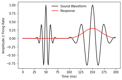
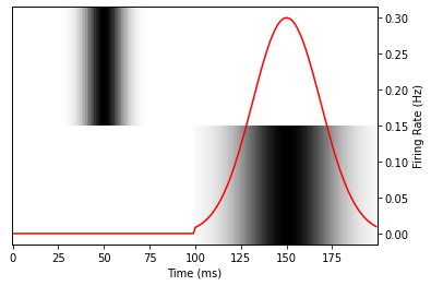
Note that our imaginary neuron doesn’t fire at all in response to the 5 KHz tone, but responds in direct proportion to the amplitude of the 2 KHz tone. We can model this simple linear behavior with a new WeightChannels Layer. In particuar, if we represent the sound waveform as a 2-channel pseudo-spectrogram, we should fit weights of 0 and 0.3 for the high- and low-frequency channels, respectively. Note that in the spectrogram generated below, frequency is represented discretely on the vertical axis and amplitude is represented by saturation

high_channel = np.concatenate([high_envelope, np.zeros_like(t)])
low_channel = np.concatenate([np.zeros_like(t), low_envelope])
spectrogram = np.vstack([high_channel, low_channel]).T

def plot_data(prediction=None):
    fig, ax = plt.subplots(1,1)
    ax2 = ax.twinx()
    ax.imshow(spectrogram.T, aspect='auto', interpolation='none', cmap='binary')
    ax2.plot(response, 'r-')
    if prediction is not None:
        ax2.plot(prediction, 'b--')

    ax.yaxis.set_visible(False)
    ax.set_xlabel("Time (ms)")
    ax2.set_ylabel("Firing Rate (Hz)")

plot_data()

Now, let’s use Model.fit to try to match the response data. We’ll create a new Layer that computes a weighted sum of the spectrogram input to predict the response. A successful fit should be able to find the correct parameter values, [0.0, 0.3]. Note that WeightChannels already exists in the nems.layers library, but we’ll re-create a simple version here to demonstrate.

class WeightChannels(Layer):
    def initial_parameters(self):
        coefficients = Parameter('coefficients', shape=self.shape)
        return Phi(coefficients)

    def evaluate(self, spectrogram):
        # Only two inputs are supported, and they are weighted differently.
        coefficients = self.get_parameter_values()
        # @ represents matrix multiplication, and the squeeze prevents an
        # extra dimension from being prepended to the output.
        return np.squeeze(spectrogram @ coefficients, axis=0)

linear_model = Model(layers=WeightChannels(shape=(2,1)))

Epoch 0
==============================
        Iteration 0, error is: 0.00758946...
Fit successful: False
Status: 2
Message: ABNORMAL_TERMINATION_IN_LNSRCH

Fitted parameter values:
{'WeightChannels': {'coefficients': array([[-3.70172149e-09],
       [ 2.99999997e-01]])}}

First, we’ll check that the model behaves as expected with some random initial parameters.

random_model = linear_model.sample_from_priors()
print(random_model.get_parameter_values()['WeightChannels']['coefficients'])
plot_data(random_model.predict(spectrogram))

[[0.14423579]
 [1.59272023]]

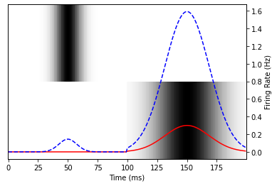
Depending on the parameters you generated, you should see that the blue curve responds strongly to the first sound if the first coefficient is large, and responds strongly to the second sound if the second coefficient is large.

Now, let’s fit to the simulated data.

fitted_model = random_model.fit(spectrogram, response)
print(f"\nFitted parameter values:\n{fitted_model.get_parameter_values()}")

Epoch 0
==============================
        Iteration 0, error is: 0.22535711...
        Iteration 5, error is: 0.00800495...
        Iteration 10, error is: 0.00023635...
        Iteration 15, error is: 0.00000697...
        Iteration 20, error is: 0.00000023...
Fit successful: False
Status: 2
Message: ABNORMAL_TERMINATION_IN_LNSRCH

Fitted parameter values:
{'WeightChannels': {'coefficients': array([[-3.12388031e-09],
       [ 3.00000000e-01]])}}

In this case we can clearly see that the fit was successful since there are only two parameter values to check. However, we can also use Model.score to get a more succinct assessment for larger models. By default, this computes the pearson correlation between the Model prediction and the target data.

fitted_model.score(spectrogram, response)

1.0

plot_data(fitted_model.predict(spectrogram))

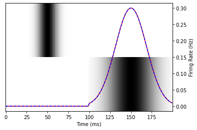
A perfect match!